Research
Jazmin Calimano Colon
2026-04-19
Part I
In this section, I will tidy the datasets containing race and income information on Young Adult Migration in the United States.
#Load libraries
pacman::p_load(tidyverse, dplyr, skimr)

#Read csv files
income <- read.csv("data/data_income.csv")
race <- read.csv("data/data_race.csv")
Tidying the race dataset.
Q1 What is the unit of observation? \[2 points\]
The unit of observation is the origin-to-destination pair, in other words, the starting and ending locations of the individuals after 10 years.
Q2 What variables are in the data? \[2 points\]
colnames(race)## [1] "unique" "o_cz_name" "o_state_name" "d_cz_name"
## [5] "d_state_name" "race" "young_adults"Q3 Is the dataset tidy? Why / Why not? \[4 points\]
The dataset is not tidy because there isn’t a single observation per row. The “unique” column contains two id variables for the origin city and destination city that could be separated into their own columns. The “race” column could also be expanded so that each categorical variable within has its own column with the corresponding population of young adults as its values.
Q4 Tidy the data_race dataset. \[6 points\]
glimpse(race)## Rows: 53,352
## Columns: 7
## $ unique <chr> "14801_4101", "14801_4101", "14801_4101", "14801_…
## $ o_cz_name <chr> "Olney", "Olney", "Olney", "Olney", "Olney", "Oln…
## $ o_state_name <chr> "Illinois", "Illinois", "Illinois", "Illinois", "…
## $ d_cz_name <chr> "Crossett", "Crossett", "Crossett", "Crossett", "…
## $ d_state_name <chr> "Arkansas", "Arkansas", "Arkansas", "Arkansas", "…
## $ race <chr> "Asian", "Black", "Hispanic", "Other", "Asian", "…
## $ young_adults <int> 0, 0, 0, 0, 0, 0, 0, 0, 0, 0, 0, 0, 0, 0, 0, 0, 0…race <- race %>%
separate(col = unique,
into = c("o_cz", "d_cz"),
sep = "_",
convert = T) %>%
pivot_wider(names_from = "race",
values_from = "young_adults")
glimpse(race)## Rows: 13,338
## Columns: 10
## $ o_cz <int> 14801, 14801, 14801, 14801, 14801, 14801, 14801, …
## $ d_cz <int> 4101, 35402, 34301, 5000, 37901, 29008, 18202, 37…
## $ o_cz_name <chr> "Olney", "Olney", "Olney", "Olney", "Olney", "Oln…
## $ o_state_name <chr> "Illinois", "Illinois", "Illinois", "Illinois", "…
## $ d_cz_name <chr> "Crossett", "Cortez", "Cody", "Tupelo", "Las Vega…
## $ d_state_name <chr> "Arkansas", "Colorado", "Wyoming", "Mississippi",…
## $ Asian <int> 0, 0, 0, 0, 0, 0, 0, 0, 0, 0, 0, 0, 0, 0, 0, 0, 0…
## $ Black <int> 0, 0, 0, 0, 0, 0, 0, 0, 0, 0, 0, 0, 0, 0, 0, 0, 0…
## $ Hispanic <int> 0, 0, 0, 0, 0, 0, 0, 0, 0, 0, 0, 0, 0, 0, 0, 0, 0…
## $ Other <int> 0, 0, 0, 0, 3, 0, 0, 0, 0, 0, 0, 0, 3, 0, 3, 0, 0…Tidying the income dataset.
Q5 What is the unit of observation? \[2 points\]
The unit of observation for this dataset is also the origin-to-destination pair.
Q6 What variables are in the data? \[2 points\]
The variables are origin city id, origin city name, origin state, destination city name, destination city id, destination state, and parental income in quantiles.
Q7 Is the dataset tidy? Why / Why not? \[4 points\]
The dataset isn’t tidy because there are more variables than observations. It can be further simplified by dividing the columns into distinct values, so that each observation is a single row.
Q8 Tidy the data_income dataset. \[8 points\]
income <- income %>%
  pivot_longer(cols = -c(o_cz, o_cz_name, o_state_name),
              names_sep = "_",
              names_to = c("d_cz", "d_cz_name", "d_state_name", "parental_income"),
               values_to = "individuals") %>%
  pivot_wider(names_from = "parental_income",
              values_from = "individuals")

glimpse(income)
## Rows: 13,338
## Columns: 11
## $ o_cz <int> 14801, 14801, 14801, 14801, 14801, 14801, 14801, …
## $ o_cz_name <chr> "Olney", "Olney", "Olney", "Olney", "Olney", "Oln…
## $ o_state_name <chr> "Illinois", "Illinois", "Illinois", "Illinois", "…
## $ d_cz <chr> "X32201", "X12800", "X28503", "X11500", "X34115",…
## $ d_cz_name <chr> "Huntsville", "Washington", "Trinidad", "Jackson"…
## $ d_state_name <chr> "Texas", "Indiana", "Colorado", "Michigan", "Alas…
## $ Q1 <int> 0, 0, 0, 0, 0, 0, 2, 0, 0, 0, 0, 0, 0, 1, 0, 0, 0…
## $ Q2 <int> 1, 0, 0, 0, 0, 0, 2, 0, 0, 0, 0, 0, 0, 0, 0, 0, 0…
## $ Q3 <int> 0, 0, 0, 0, 0, 0, 0, 0, 0, 0, 0, 0, 0, 2, 0, 0, 0…
## $ Q4 <int> 0, 0, 0, 0, 0, 0, 3, 0, 0, 0, 0, 0, 0, 4, 1, 0, 2…
## $ Q5 <int> 0, 0, 0, 0, 0, 0, 0, 0, 0, 1, 0, 0, 1, 1, 0, 0, 0…BONUS QUESTION. Try to change the structure of data_income and make the “city” the unit of analysis (e.g., each row should represent an origin city in Illinois). \[5 points\] Use these two arguments in the pivot_wider function: • id_cols • values_fn
income %>%
  pivot_wider(id_cols = starts_with("o"),
              names_from = c("d_cz", "d_cz_name", "d_state_name"),
              values_from = c("Q1", "Q2", "Q3", "Q4", "Q5"),
              values_fn = NULL)
## # A tibble: 18 × 3,708
## o_cz o_cz_name o_state_name Q1_X32201_Huntsville_Texas
## <int> <chr> <chr> <int>
## 1 14801 Olney Illinois 0
## 2 23301 Charleston Illinois 2
## 3 23302 Douglas Illinois 0
## 4 23400 Bloomington Illinois 0
## 5 23500 Decatur Illinois 0
## 6 23700 Galesburg Illinois 0
## 7 23801 Davenport Illinois 0
## 8 23900 Peoria Illinois 1
## 9 24200 Bourbonnais Illinois 0
## 10 24300 Chicago Illinois 4
## 11 24400 Rockford Illinois 1
## 12 24801 Jacksonville Illinois 0
## 13 24802 Springfield Illinois 0
## 14 24900 Edwardsville Illinois 1
## 15 25000 Quincy Illinois 0
## 16 25500 Centralia Illinois 1
## 17 25601 Carbondale Illinois 0
## 18 25602 Harrisburg Illinois 0
## # ℹ 3,704 more variables: Q1_X12800_Washington_Indiana <int>,
## # Q1_X28503_Trinidad_Colorado <int>,
## # Q1_X11500_Jackson_Michigan <int>, Q1_X34115_Fairbanks_Alaska <int>,
## # Q1_X10502_Starkville_Mississippi <int>,
## # Q1_X25701_Cape.Girardeau_Missouri <int>,
## # Q1_X32403_Snyder_Texas <int>, Q1_X34111_Ketchikan_Alaska <int>,
## # Q1_X3500_Baton.Rouge_Louisiana <int>, …Part II
Use migrationflows_tidy and population_tidy datasets for this part.
migrationflows <- read.csv("data/migrationflows_tidy.csv")
population <- read.csv("data/population_tidy.csv")
Join
Q1 Join the two datasets so that all information in population_tidy dataset are kept. Remember to follow the steps discussed in class to check if the two datasets are correctly joined. How many rows do you expect the joined dataset to have? \[6 points\]
I expect to have 1392 rows if I want to keep all observations from the population dataset. There are 3 columns in common so only 3 new columns will be added to the joined dataset.
dim(population)## [1] 1392 6dim(migrationflows)## [1] 1392 6data_joined <- left_join(population, migrationflows)## Joining with `by = join_by(Country, Country.code, year)`dim(data_joined)## [1] 1392 9Dollar-sign Syntax
Use the newly created/joined dataset to answer the following. Use dollar-sign syntax and logical indexing (i.e., []). DO NOT use dplyr functions. You will not receive points for using dplyr functions even if the output is correct.
Q2 What is the average percentage of migrants on the total population of a country in 2015? When calculating the percentage column, pay attention that population data are recorded in thousands while migration data are absolute numbers (see codebook at the beginning). \[6 points\]
The average percent of migrants on the total population of a country in 2015 is 13%
data_joined$percent_migrant <- (data_joined$Tot/(data_joined$Pop*1000)*100)

avg_2015 <- mean(data_joined$percent_migrant[data_joined$year == 2015])
avg_2015
## [1] 13.33353Q3 Did the average percentage of immigrants on the total of population increased or decreased from 1990? \[4 points\]
The average percentage of immigrants increased from 1990 to 2015.
avg_1990 <- mean(data_joined$percent_migrant[data_joined$year == 1990], na.rm = TRUE)
avg_1990
## [1] 12.69894Q4 What is the percentage change of the average number of immigrants across all countries between 1990 and 2015? Answer this question using R objects so that your code can be reproduced even if the dataset will change in the future. \[6 points\]
percent_change <- ((avg_2015 - avg_1990)/avg_1990) * 100
percent_change
## [1] 4.997221***Q5 Which is the highest percentage of male immigrants on the total in 2010? \[4 points***\]
#What is the highest percentage of male immigrants among/relative to the total immigrants in 2010?
data_joined$percent_male_immigrant <- (data_joined$Male/data_joined$Tot)*100

male_immigrants <- subset(data_joined, year == "2010", select=c(Country, percent_male_immigrant, year))

max_immigrants <- max(male_immigrants$percent_male_immigrant, na.rm = TRUE)
max_immigrants
## [1] 86.54145Q6 What is the median percentage of immigrants across all countries in 2015? \[4 points\]
percent_median <- median(data_joined$percent_migrant[data_joined$year == "2015"], na.rm = TRUE)
percent_median
## [1] 5.440095Part III
Use the migration_region dataset in this part.
migration_region <- read.csv("data/migration_region.csv")DPLYR
Use dplyr functions to answer the following questions.
Q1 What is the number of Migrant by region in 2015? \[4 points\]
migration_region %>%
  filter(year == "2015") %>%
  group_by(region) %>%
  summarise(total_migrants = sum(Migrants, na.rm = TRUE))
## # A tibble: 6 × 2
## region total_migrants
## <chr> <int>
## 1 Africa 20648953
## 2 Asia 72781741
## 3 Developed countries 140393231
## 4 Latam 9024966
## 5 Oceania 229158
## 6 Territories/Others 622187Q2 How many countries have a share of immigrants that it’s greater than or equal to 50% of their population in 2015? \[4 points\]
migration_region %>%
  filter(Migrants >= (Pop*.5)) %>%
  summarise(n_countries = n())
## n_countries
## 1 81Q3 In which world regions are most of these countries located? \[4 points\]
migration_region %>%
  filter(Migrants >= (Pop*.5)) %>%
  group_by(region) %>%
  summarise(n_countries = n())
## # A tibble: 5 × 2
## region n_countries
## <chr> <int>
## 1 Asia 26
## 2 Developed countries 16
## 3 Latam 8
## 4 Oceania 1
## 5 Territories/Others 30Q4 How many countries have a share of immigrants greater than or equal to 50% of their population if we consider the average from 1990 to 2015? \[4 points\]
migration_region %>%
  filter(year >= 1990 & year <= 2015) %>%
  mutate(migrants_per_pop = Migrants / Pop) %>%
  group_by(Country) %>%
  summarise(avg_share = mean(migrants_per_pop, na.rm = TRUE)) %>%
  filter(avg_share >= 0.5) %>%
  summarise(n_countries = n())
## # A tibble: 1 × 1
## n_countries
## <int>
## 1 14Q5 Which region saws the largest increase in the number of refugees from 1990 to 2015? And which region saws the largest decrease? \[6 points\]
Asia had the largest increase in the number of refugees (2140863). And Africa had the largest decrease in refugees (-1905662).
migration_region %>%
  select(Country, year, Refugees, region) %>%
  filter(year %in% c("1990", "2015")) %>%
  group_by(region, year) %>%
  summarise(yearly_refugees = sum(Refugees, na.rm = TRUE)) %>%
  pivot_wider(names_from = year,
              values_from = yearly_refugees) %>%
  mutate(change = `2015` - `1990`) %>%
  arrange(desc(change))
## # A tibble: 6 × 4
## # Groups: region [6]
## region `1990` `2015` change
## <chr> <int> <int> <int>
## 1 Asia 9019721 11160584 2140863
## 2 Territories/Others 910637 2051532 1140895
## 3 Oceania 7099 4812 -2287
## 4 Developed countries 2014564 1947064 -67500
## 5 Latam 1197198 383956 -813242
## 6 Africa 5687352 3781690 -1905662Q6 Has there been any changes in the immigration patterns by gender over time? Consider the average across all the years. \[4 points\]
Yes, the results in the table below show that for both genders the immigration patterns have been increasing over the years.
migration_region %>%
  select(year, MaleMigrants, FemaleMigrants) %>%
  group_by(year) %>%
  summarise(avg_male = mean(MaleMigrants, na.rm = T), avg_female = mean(FemaleMigrants, na.rm = T))
## # A tibble: 6 × 3
## year avg_male avg_female
## <int> <dbl> <dbl>
## 1 1990 340998. 328139.
## 2 1995 358498. 346773.
## 3 2000 385460. 372011.
## 4 2005 427365. 407871.
## 5 2010 494025. 461640.
## 6 2015 543601. 506831.Missing values
Q7 Use the is.na functions to calculate how many missing values in the refugees, population, and migrant columns. \[4 points\]
sum(is.na(migration_region$Refugees))## [1] 366sum(is.na(migration_region$Pop))## [1] 0sum(is.na(migration_region$Migrants))## [1] 15Q8 For the column(s) with missing values, conduct some additional analysis- are those random by region, year, or country? Which regions, years, or countries have the largest amount of missing values? Can you think of an explanation of why there are these missing values? Would you classify these missing values as MCAR, MAR, or MNAR? \[6 points\]
Region with largest missing values: Territories/Other
Because these are small nations and territories, it could be that they do not have the resources to either support refugees or accurately count the number of refugees or migrants in their country. The countries belonging to Territories/Other also have the lowest average population. I would then categorize these missing values sharing this common characteristic as missing at random.
#total missing values from refugees (366) and migrants (15)
migration_region %>%
  group_by(region) %>%
  summarise(
    miss_refugees = sum(is.na(Refugees)),
    miss_migrants = sum(is.na(Migrants))
  )
## # A tibble: 6 × 3
## region miss_refugees miss_migrants
## <chr> <int> <int>
## 1 Africa 54 4
## 2 Asia 42 0
## 3 Developed countries 24 4
## 4 Latam 48 0
## 5 Oceania 42 0
## 6 Territories/Others 156 7migration_region %>%
group_by(Country) %>%
summarise(
miss_refugees = sum(is.na(Refugees)),
miss_migrants = sum(is.na(Migrants))
) %>%
filter(miss_refugees >0 | miss_migrants >0)## # A tibble: 62 × 3
## Country miss_refugees miss_migrants
## <chr> <int> <int>
## 1 American Samoa 6 0
## 2 Andorra 6 0
## 3 Anguilla 6 0
## 4 Antigua and Barbuda 6 0
## 5 Aruba 6 0
## 6 Barbados 6 0
## 7 Bermuda 6 0
## 8 Bhutan 6 0
## 9 Bonaire, Sint Eustatius and Saba 6 0
## 10 Brunei Darussalam 6 0
## # ℹ 52 more rowsmigration_region %>%
group_by(region, year, Country) %>%
summarise(
miss_refugees = sum(is.na(Refugees)),
miss_migrants = sum(is.na(Migrants))
) %>%
filter(miss_refugees >0 | miss_migrants >0) %>%
arrange(Country)## `summarise()` has grouped output by 'region', 'year'. You can override
## using the `.groups` argument.## # A tibble: 370 × 5
## # Groups: region, year [36]
## region year Country miss_refugees miss_migrants
## <chr> <int> <chr> <int> <int>
## 1 Territories/Others 1990 American Samoa 1 0
## 2 Territories/Others 1995 American Samoa 1 0
## 3 Territories/Others 2000 American Samoa 1 0
## 4 Territories/Others 2005 American Samoa 1 0
## 5 Territories/Others 2010 American Samoa 1 0
## 6 Territories/Others 2015 American Samoa 1 0
## 7 Developed countries 1990 Andorra 1 0
## 8 Developed countries 1995 Andorra 1 0
## 9 Developed countries 2000 Andorra 1 0
## 10 Developed countries 2005 Andorra 1 0
## # ℹ 360 more rowsmigration_region %>%
group_by(region) %>%
summarise(total = mean(Pop))## # A tibble: 6 × 2
## region total
## <chr> <dbl>
## 1 Africa 15545611.
## 2 Asia 76366080.
## 3 Developed countries 24472782.
## 4 Latam 15069144.
## 5 Oceania 825583.
## 6 Territories/Others 146609.Q9 Write a short wrap-up of what you discovered on missing values. Note any surprising findings and you think missing values might affect any analysis contacted with the dataset. \[4 points\]
The Territories/Others category has the most number of missing values, and surprisingly, the exact number of missing values per region/country are consistent each year from 1990 to 2015. Most of these are territories belonging to other nations, so it could be that these values have been either undercounted or included in their colonizer’s migrant and refugee count. I do not think these missing values will have a large effect on the analyses conducted on the dataset because they are being omitted. And it will be necessary to clarify why these values were missing and omitted from the final result.
PART IV
Load the data file called car_data.csv. This data contains information about cars and motorcycles listed on CarDekho.com.
car_data <- read.csv("data/car_data.csv")
library(hrbrthemes)
Visualization
Q1 Explore and describe the distribution of the selling price using the appropriate graph. Add a vertical line indicating the mean selling price on the same graph. \[4 points\]
glimpse(car_data)## Rows: 4,340
## Columns: 8
## $ name <chr> "Maruti 800 AC", "Maruti Wagon R LXI Minor", "Hy…
## $ year <int> 2007, 2007, 2012, 2017, 2014, 2007, 2016, 2014, …
## $ selling_price <int> 60000, 135000, 600000, 250000, 450000, 140000, 5…
## $ km_driven <int> 70000, 50000, 100000, 46000, 141000, 125000, 250…
## $ fuel <chr> "Petrol", "Petrol", "Diesel", "Petrol", "Diesel"…
## $ seller_type <chr> "Individual", "Individual", "Individual", "Indiv…
## $ transmission <chr> "Manual", "Manual", "Manual", "Manual", "Manual"…
## $ owner <chr> "First Owner", "First Owner", "First Owner", "Fi…car_data %>%
ggplot(mapping = aes(selling_price)) +
geom_histogram(bins = 100, fill="orange") +
geom_vline(aes(xintercept = mean(selling_price))) +
theme_minimal() +
ggtitle("Mean Selling Price of Cars and Motorcycles = 504127")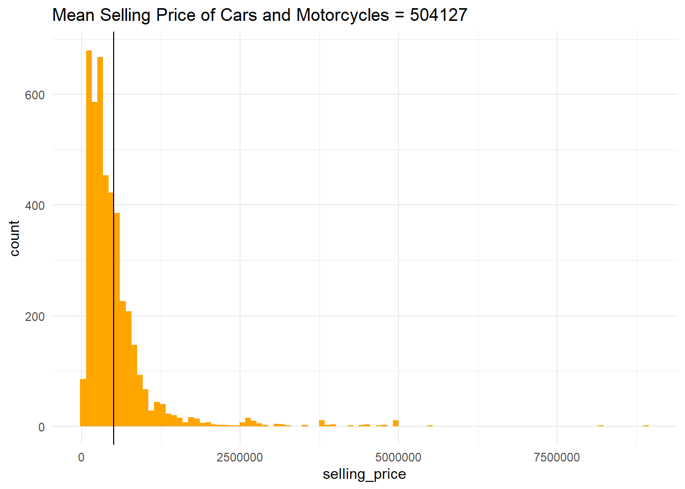
Q2 Create a correlogram among selling price, number of kilometers driven, and year the car was bought using the appropriate function in the GGally package. [6 points}
library(GGally)## Warning: package 'GGally' was built under R version 4.5.2ggpairs(car_data, columns = 2:4, ggplot2::aes(colour=owner)) +
theme_bw()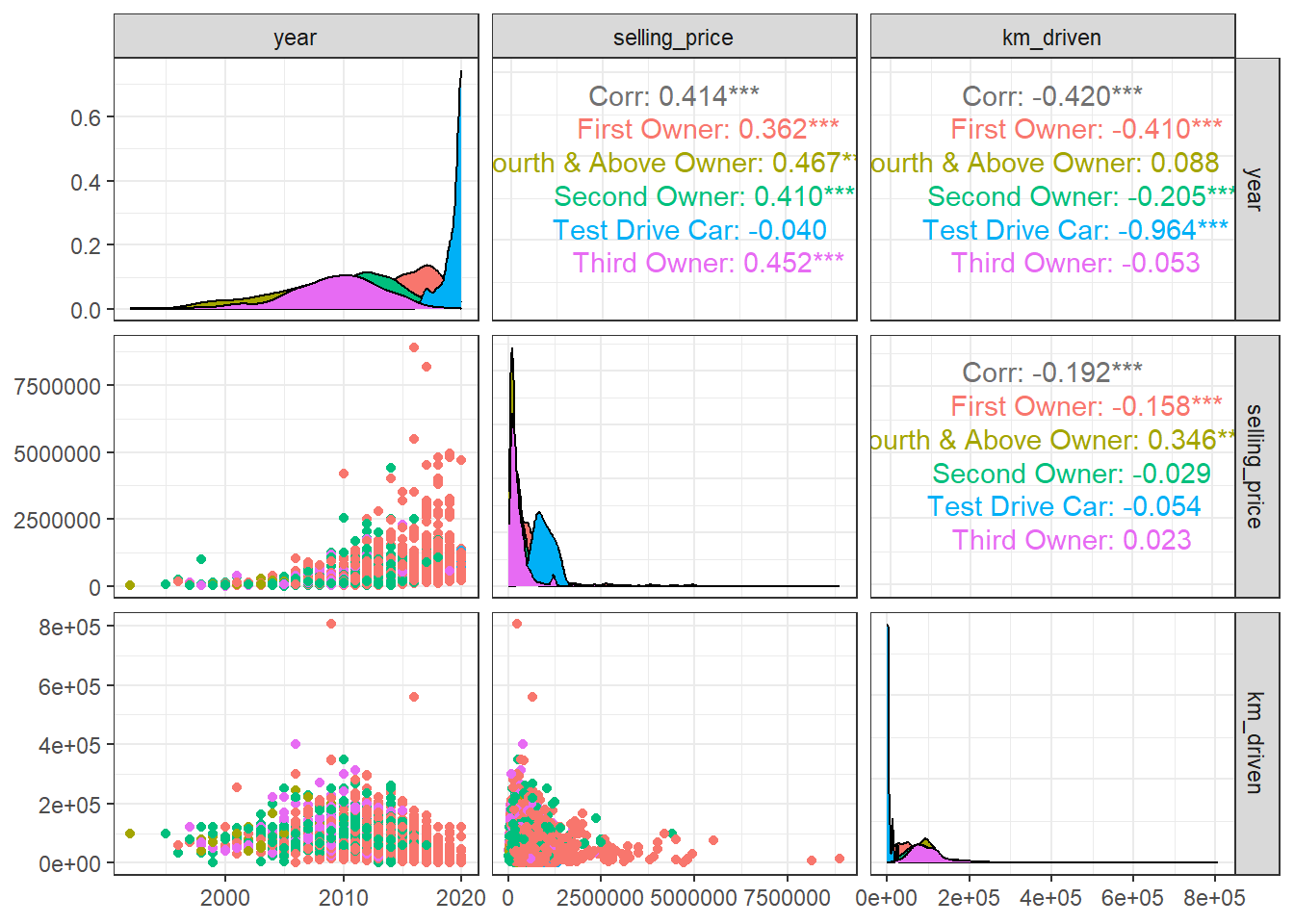
Q3 Plot the relationship between the selling price and year for the automatic and manual cars on the same plot. (4 points). The points on the graph should be colored based on transmission (2 points), and the tooltip should indicate the year, selling price, and transmission type. (3 points)
library(plotly)

p <- car_data %>%
  ggplot(aes(x = year, y = selling_price, color = transmission)) +
    geom_point(alpha=0.7) +
  theme_classic() +
  labs(title = "Selling price and year for automatic and manual cars")

ggplotly(p)